Bi-Objective GEBV Selection Pareto Frontier Visualization#
Selection of individuals based on their genomic estimated breeding values (GEBVs) is a common task in a breeding program implementing genomic selection. In this example, we demonstrate how to optimize and visualize an estimate of the Pareto frontier for a bi-objective GEBV selection problem in a subset search space. In the bi-objective GEBV selection problem, we seek to maximize the mean GEBV of a selected subset of individuals from a set of candidates for two traits simultaneously.
Loading Required Modules and Seeding the Global Random Number Generator#
To begin, we import the modules we will be using into the Python namespace. To make our simulation replicable, we set the seed for the simulation using the seed function in the pybrops.core.random.prng module. This seeds the Python random and NumPy numpy.random modules with a single seed.
# import libraries
import numpy
from matplotlib import pyplot
import pybrops
from pybrops.breed.prot.sel.GenomicEstimatedBreedingValueSelection import GenomicEstimatedBreedingValueSubsetSelection
from pybrops.opt.algo.NSGA2SubsetGeneticAlgorithm import NSGA2SubsetGeneticAlgorithm
from pybrops.model.gmod.DenseAdditiveLinearGenomicModel import DenseAdditiveLinearGenomicModel
from pybrops.popgen.gmat.DenseGenotypeMatrix import DenseGenotypeMatrix

# seed python random and numpy random
pybrops.core.random.prng.seed(31621463)
Loading Genotypic Data from a VCF File#
Next, we load our genotypic data from a VCF file named "widiv_2000SNPs.vcf.gz" using the from_vcf class method in the DenseGenotypeMatrix class. This creates an unphased genotype matrix with our SNPs coded as 0, 1, and 2. We automatically sort and group the genetic variants in the genotype matrix based on their chromosome assignments and physical positions using the auto_group_vrnt = True option.
# read unphased genetic markers from a vcf file
gmat = DenseGenotypeMatrix.from_vcf(
    "widiv_2000SNPs.vcf.gz", # file name to load
    auto_group_vrnt = True,  # automatically sort and group variants
)
Constructing a Bi-Trait Genomic Model#
Next, we construct a genomic model. The user may construct a genomic model by any means, including loading a model from file(s). Here, we simply construct a random bi-trait genomic model to represent two synthetic traits.
Below, we draw marker effects from a bi-variate normal distribution with negative covariance. This in effect, creates two traits with pleiotrophic effects which are competing in nature.
# make marker effects for two traits which are competing in nature
# marker effects array is of shape (nvrnt, 2)
mkreffect = numpy.random.multivariate_normal(
    mean    = numpy.array([0.0, 0.0]),
    cov     = numpy.array([
                [ 1.0, -0.4],
                [-0.4,  1.0]
            ]),
    size    = gmat.nvrnt
)
Below, we construct a genomic model from our randomly drawn marker effects to make the genomic model that we will use to calculate GEBVs.
# create an additive linear genomic model to model traits
algmod = DenseAdditiveLinearGenomicModel(
    beta    = numpy.float64([[10.0, 25.0]]), # model intercepts
    u_misc  = None,                          # miscellaneous random effects
    u_a     = mkreffect,                     # random marker effects
    trait   = numpy.array(                   # trait names
                ["syn1","syn2"],
                dtype=object
            ),
    model_name = "synthetic_model",          # name of the model
    hyperparams = None                       # model parameters
)
Constructing a GEBV Subset Selection object#
After constructing a genomic model, our next step is to create a selection protocol that will construct selection problems and optimize them for use, given genotype matrix and genomic model inputs.
Since the subset search space is large (there are 942 candidate individuals from which to choose), we’ll want to provide a multi-objective optimization algorithm different from the default that will be able to optimize our GEBV selection problem. We’ll make a slight variation on the default NSGA2SubsetGeneticAlgorithm and increase the number of algorithm generations from 250 to 1000.
# create custom multi-objective algorithm for optimization
# use NSGA-II and evolve for 1000 generations
moalgo = NSGA2SubsetGeneticAlgorithm(
    ngen = 1000,    # number of generations to evolve
    pop_size = 100  # number of parents in population
)
Next, we’ll construct a GEBV selection protocol object. For this example, we desire to select 10 pairs of individuals (20 individuals total) from the 942 candidates. The code below demonstrates how this object is constructed.
# construct a subset selection object for GEBV selection
selprot = GenomicEstimatedBreedingValueSubsetSelection(
    ntrait = 2,         # number of traits to expect from GEBV matrix
    unscale = True,     # unscale GEBVs so that units are in unscaled trait values
    ncross = 10,        # number of breeding crosses to select
    nparent = 2,        # number of parents per breeding cross to select
    nmating = 1,        # number of times parents are mated per cross
    nprogeny = 40,      # number of progenies to derive from a mating event
    nobj = 2,           # number of objectives (ntrait)
    moalgo = moalgo,    # custom multi-objective algorithm
)
Estimating the Pareto Frontier#
Using the GEBV selection protocol object we just constucted, we’ll use the mosolve method to perform a multi-objective optimization to maximize the mean GEBV for both of our synthetic traits in the selected subset of individuals. The GenomicEstimatedBreedingValueSubsetSelection.mosolve method only requires two non-None arguments: gmat and gpmod. We pass our genotype matrix and genomic model objects as arguments for these two parameters, leaving the other arguments None or 0.
# estimate pareto frontier using optimization algorithm
selsoln = selprot.mosolve(
    pgmat = None,       # argument not utilized
    gmat = gmat,        # ``gmat`` argument required
    ptdf = None,        # argument not utilized
    bvmat = None,       # argument not utilized
    gpmod = algmod,     # ``gpmod`` argument required
    t_cur = 0,          # argument not utilized
    t_max = 0,          # argument not utilized
)
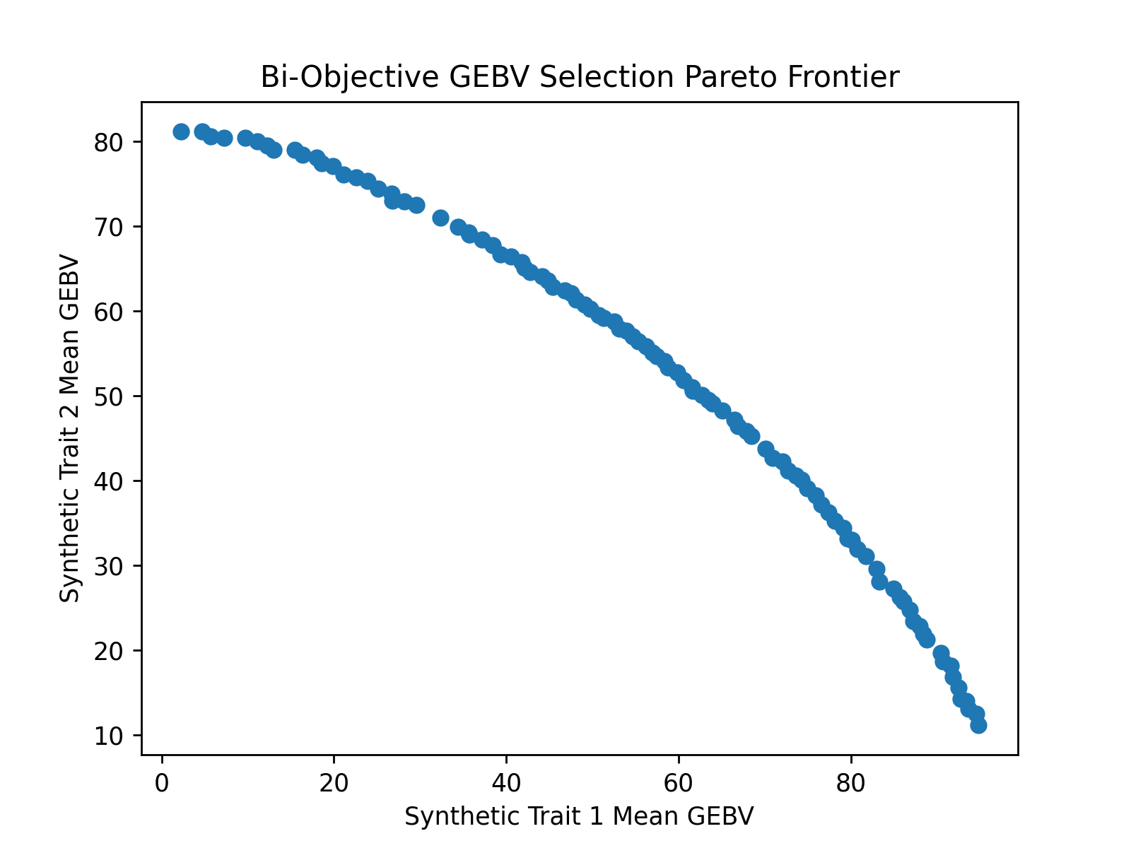
Visualizing the Pareto Frontier with matplotlib#
After optimizing the objectives, we can use matplotlib or any other plotting packages to visualize the results of the optimization. The code below creates a figure to visualize the estimated Pareto frontier.
# get the pareto frontier
# negate the objectives to get the mean GEBV since optimization problems are always minimizing
xdata = -selsoln.soln_obj[:,0]
ydata = -selsoln.soln_obj[:,1]

# create static figure
fig = pyplot.figure()
ax = pyplot.axes()
ax.scatter(xdata, ydata)
ax.set_title("Bi-Objective GEBV Selection Pareto Frontier")
ax.set_xlabel("Synthetic Trait 1 Mean GEBV")
ax.set_ylabel("Synthetic Trait 2 Mean GEBV")
pyplot.savefig("biobjective_GEBV_pareto_frontier.png", dpi = 250)
pyplot.close(fig)
Below is the image which was created by matplotlib.