Tri-Objective Optimal Contribution Selection Pareto Frontier Visualization#
Optimial Contribution Selection (OCS) is a diversity preservation strategy commonly used in breeding. In OCS, the breeding value of a selected subset of individuals is maximized subject to an inbreeding constraint. This optimization can be generalized to a multi-objective scenario where one or more breeding values are maximized and inbreeding level is minimized, simultaneously. In this example, we demonstrate how to optimize and visualize an estimate of the Pareto frontier for a tri-objective OCS problem in a subset search space. In the tri-objective OCS problem, we seek to maximize the estimated breeding values (EBVs) for two traits and minimize the inbreeding between individuals in the selected subset, simultaneously.
Loading Required Modules and Seeding the global PRNG#
To begin, we import the modules we will be using into the Python namespace. To make our simulation replicable, we set the seed for the simulation using the seed function in the pybrops.core.random.prng module. This seeds the Python random and NumPy numpy.random modules with a single seed. We’ll also want to import some image processing libraries such as matplotlib and PIL.
# import libraries
import os
import numpy
from matplotlib import pyplot
from matplotlib import rcParams
rcParams['font.family'] = 'Liberation Serif' # set default font
from PIL import Image
import pybrops
from pybrops.breed.prot.sel.OptimalContributionSelection import OptimalContributionSubsetSelection
from pybrops.opt.algo.NSGA3SubsetGeneticAlgorithm import NSGA3SubsetGeneticAlgorithm
from pybrops.model.gmod.DenseAdditiveLinearGenomicModel import DenseAdditiveLinearGenomicModel
from pybrops.popgen.gmat.DenseGenotypeMatrix import DenseGenotypeMatrix
from pybrops.popgen.cmat.fcty.DenseMolecularCoancestryMatrixFactory import DenseMolecularCoancestryMatrixFactory

# seed python random and numpy random
pybrops.core.random.prng.seed(31621463)
Loading Genotypic Data from a VCF File#
Next, we load our genotypic data from a VCF file named "widiv_2000SNPs.vcf.gz" using the from_vcf class method in the DenseGenotypeMatrix class. This creates an unphased genotype matrix with our SNPs coded as 0, 1, and 2. We automatically sort and group the genetic variants in the genotype matrix based on their chromosome assignments and physical positions using the auto_group_vrnt = True option.
# read unphased genetic markers from a vcf file
gmat = DenseGenotypeMatrix.from_vcf(
    "widiv_2000SNPs.vcf.gz", # file name to load
    auto_group_vrnt = True,  # automatically sort and group variants
)
Constructing a Bi-Trait Genomic Model#
Next, we construct a genomic model. The user may construct a genomic model by any means, including loading a model from file(s). Here, we simply construct a random bi-trait genomic model to represent two synthetic traits.
Below, we draw marker effects from a bi-variate normal distribution with negative covariance. This in effect, creates two traits with pleiotrophic effects which are competing in nature.
# make marker effects for two traits which are competing in nature
# marker effects array is of shape (nvrnt, 2)
mkreffect = numpy.random.multivariate_normal(
    mean    = numpy.array([0.0, 0.0]),
    cov     = numpy.array([
                [ 1.0, -0.4],
                [-0.4,  1.0]
            ]),
    size    = gmat.nvrnt
)
# create an additive linear genomic model to model traits
algmod = DenseAdditiveLinearGenomicModel(
    beta    = numpy.float64([[10.0, 25.0]]), # model intercepts
    u_misc  = None,                          # miscellaneous random effects
    u_a     = mkreffect,                     # random marker effects
    trait   = numpy.array(                   # trait names
                ["syn1","syn2"],
                dtype=object
            ),
    model_name = "synthetic_model",          # name of the model
    hyperparams = None                       # model parameters
)
Constructing a Breeding Value Matrix#
Next, we construct a breeding value matrix using our genomic model. The breeding value matrix will be used directly by the optimal contribution selection protocol in the steps following. Here, the user may construct a breeding value matrix by any means, including loading it from a file.
# calculate the GEBVs from the genotype matrix
bvmat = algmod.gebv(gtobj = gmat)
Constructing an Optimal Contribution Subset Selection Object#
Next, we construct a CoancestryMatrixFactory object. The purpose of this object is to generate coancestry matrices from genotype matrices. The code below creates a factory object that will generate identity by state coancestry matrices. Other factory objects can be substituted here (e.g. VanRaden genomic relationship matrix, Yang genomic relationship matrix factory objects) to customize the OCS selection protocol object.
# create coancestry matrix factory object for creating
# identity by state coancestry matrices
ibscmatfcty = DenseMolecularCoancestryMatrixFactory()
Since the subset search space is large (there are 942 candidate individuals from which to choose), we’ll want to provide a multi-objective optimization algorithm different from the default that will be able to optimize our weighted genomic selection problem. We’ll make a slight variation on the default NSGA2SubsetGeneticAlgorithm and increase the number of algorithm generations from 250 to 1000.
# create custom multi-objective algorithm for optimization
algo = NSGA3SubsetGeneticAlgorithm(
    ngen = 1500,    # number of generations to evolve
    pop_size = 100, # number of parents in population
    nrefpts = 91,   # number of reference points for optimization
)
Next, we’ll construct an optimal contribution selection protocol object. For this example, we desire to select 10 pairs of individuals (20 individuals total) from the 942 candidates in the genotype matrix. The code below demonstrates how this object is constructed.
# construct a subset selection problem for OCS
selprot = OptimalContributionSubsetSelection(
    ntrait = 2,             # number of expected traits
    cmatfcty = ibscmatfcty, # identity by state
    unscale = True,         # whether to unscale breeding values
    ncross = 10,            # number of breeding crosses to select
    nparent = 2,            # number of parents per breeding cross to select
    nmating = 1,            # number of times parents are mated per cross
    nprogeny = 40,          # number of progenies to derive from a mating event
    nobj = 3,               # number of objectives (1+ntrait)
    moalgo = algo,          # custom multi-objective algorithm
    # leave all other arguments as their default values
)
Estimating the Pareto Frontier#
Using the optimal contribution selection protocol object we just constucted, we’ll use the mosolve method to perform a multi-objective optimization to maximize the mean EBVs for both of our synthetic traits and minimize the inbreeding relationship in the selected subset of individuals. The OptimalContributionSubsetSelection.mosolve method only requires two non-None arguments: gmat and bvmat. We pass our genotype matrix and breeding value matrix objects as arguments for these two parameters, leaving the other arguments None or 0.
# estimate pareto frontier
selsoln = selprot.mosolve(
    pgmat = None,   # argument not utilized
    gmat = gmat,    # ``gmat`` argument required
    ptdf = None,    # argument not utilized
    bvmat = bvmat,  # ``bvmat`` argument required
    gpmod = None,   # argument not utilized
    t_cur = 0,      # argument not utilized
    t_max = 0,      # argument not utilized
)
Visualizing the Pareto Frontier with matplotlib#
Creating a static image#
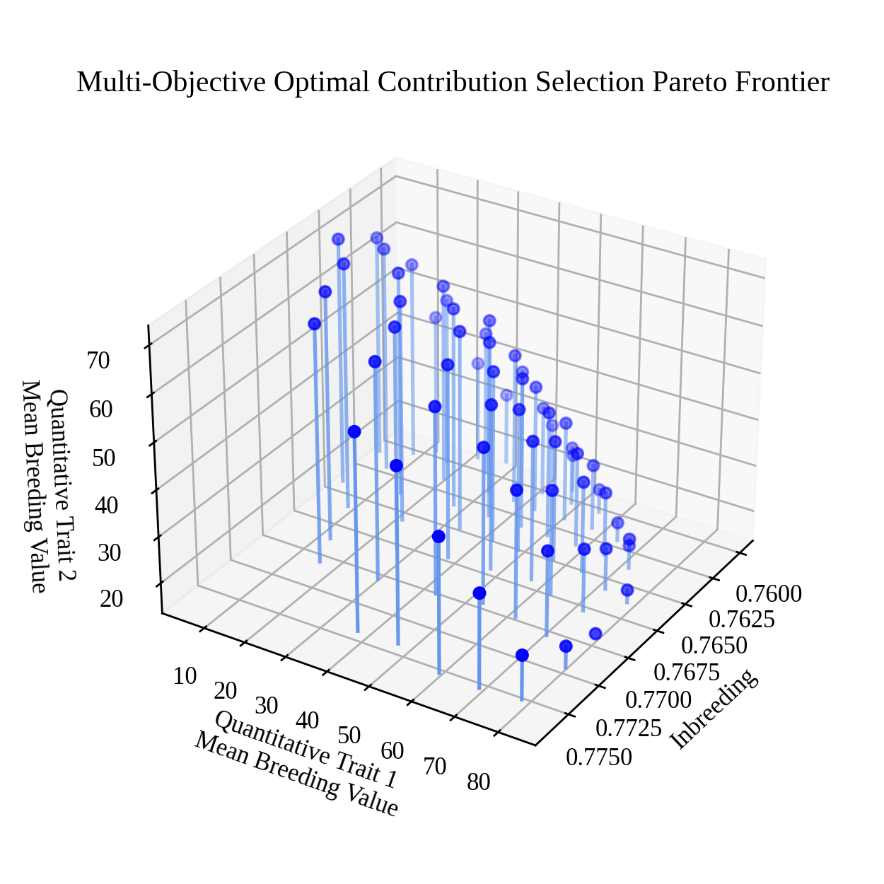
After optimizing the objectives, we can use matplotlib or any other plotting packages to visualize the results of the optimization. The code below creates a figure to visualize the estimated Pareto frontier.
# set default font size
rcParams['font.size'] = 10

# image base name
basename = "triobjective_OCS_pareto_frontier"

# get axis data
x =  selsoln.soln_obj[:,0] # 2 * mean kinship (additive relationship/inbreeding)
y = -selsoln.soln_obj[:,1] # negate to get Breeding Value
z = -selsoln.soln_obj[:,2] # negate to get Breeding Value
z2 = numpy.ones(shape = x.shape) * min(z)

# create static figure
fig = pyplot.figure(figsize=(5,5))
ax = pyplot.axes(projection = "3d")
ax.scatter(x, y, z, color = "blue")
for i,j,k,h in zip(x,y,z,z2):
    a = 0.5 * (i - min(x)) / (max(x) - min(x)) + 0.5
    ax.plot([i,i],[j,j],[k,h], color="cornflowerblue", alpha = a)

ax.set_title("Multi-Objective Optimal Contribution Selection Pareto Frontier")
ax.set_xlabel("Inbreeding")
ax.set_ylabel("Quantitative Trait 1\nMean Breeding Value")
ax.set_zlabel("Quantitative Trait 2\nMean Breeding Value")
ax.view_init(elev = 30., azim = 32)
pyplot.savefig(basename + ".png", dpi = 250)
pyplot.close(fig)
Below is the resulting figure:
Creating an animation#
Since there are three objectives, visualization of the estimated Pareto frontier may be difficult to see from a single vantage point. We can create an animation using the PIL library or other packages. The code below creates an animation to visualize the estimated Pareto frontier in 3D space.
# set default font size
rcParams['font.size'] = 10

# image base name
basename = "triobjective_OCS_pareto_frontier"

# create animation frames output directory
outdir = "frames"
if not os.path.isdir(outdir):
    os.mkdir(outdir)

# create animation frames
for i in range(360):
    fig = pyplot.figure()
    ax = pyplot.axes(projection = '3d')
    ax.scatter3D(x, y, z)
    ax.set_title("Multi-Objective Optimal Contribution Selection Pareto Frontier")
    ax.set_xlabel("Inbreeding")
    ax.set_ylabel("Quantitative Trait 1\nMean Breeding Value")
    ax.set_zlabel("Quantitative Trait 2\nMean Breeding Value")
    ax.view_init(elev = 30., azim = i)
    pyplot.savefig(outdir + "/" + basename + "_" + str(i).zfill(3) + ".png", dpi = 250)
    pyplot.close(fig)

# construct filenames from which to read
filenames = [outdir + "/" + basename + "_" + str(i).zfill(3) + ".png" for i in range(360)]

# read image files from which to create animation using PIL
images = [Image.open(filename) for filename in filenames]

# resize images to 50% size using PIL
images_resize = [img.resize(tuple(px // 2 for px in img.size)) for img in images]

# get first image
img = images_resize[0]

# create gif by appending remaining images to end of first image
img.save(
    basename + ".gif",
    save_all = True,
    append_images = images_resize[1:],
    optimize = True,
    duration = 55,      # inverse of speed
    loop = 0,           # loop indefinitely
)
Below is the resulting animation: